Difference from Static Correlation

What is a living correlation? How does it differ from the regular statistical correlation. What does it mean for a numerical entity like this to be alive? What is the significance of this unusual concept? Is it just a mathematical abstraction? Or does it have some pragmatic function? To understand the importance of this novel concept, we will first explore the mathematical meaning of a static correlation - the type employed by scientists all over the globe.

In traditional statistics, behavioral scientists compute the correlation coefficient to determine the relationship between two ordered data sets. If the coefficient is 1, then it is said that there is a positive correlation between the sets. Both data sets rise and fall together identically. If the coefficient is -1, then it is said that there is an inverse correlation between the two sets. When one data set rises, the other falls, and vice versa. If the coefficient is 0, then it is said that there is no correlation between the sets.

If the 2 data sets are smaller subsets of larger sets, then the correlation coefficient enables scientists to make predictions within predefined limits about the behavior of the set members in relationship to each other. For instance, if there is a positive correlation between the subsets, a large element of one set will tend to correspond with a large element of the other set. In this sense, correlations ultimately enable scientists to make predictions about behavior.

There are very precise mathematical rules regarding these predictions. The number of elements in the subset, the distribution of the subset, and the method of choosing the elements of the subset are just a few of the factors that must be taken into account when evaluating the precision of the prediction. There are yet other factors that must be taken into account when evaluating the significance of the prediction.

Scientists require fixed data sets to evaluate each of these standards. This allows them to make definitive statements regarding the nature of a multiplicity of populations and their relationships to each other. Indeed students spend years studying these exceedingly complicated mathematical laws of probability and statistics in order to eventually become professors. They will then publish papers that take these laws of statistics into account when drawing conclusions about living systems.

Living systems don’t have the luxury of time and study when making their predictions regarding survival. Most decisions are made on the spot. Rough guesstimates are made that enable them to avoid becoming food, procure sustenance and find sexual partners.

On the most basic level, these rough guesstimates involve the behavior of environmental data stream. Due to time and memory constraints, organisms must base their predictions upon what went just before, rather than upon the elements of an entire data set. We’ve demonstrated elsewhere that the Living Algorithm generates up-to-date information regarding the moment-to-moment nature of a data stream. These include measures that determine the location, range and tendency of the data stream from point to point. Living systems could easily employ these descriptive measures as predictors to extend their existence. Knowledge of these figures would certainly enable them to better survive the vicissitudes of fate.

Due to the need for immediate predictors applied to a rapidly and regularly changing world, these living measures are rough predictors of data stream behavior. Precision must be sacrificed for immediacy. However any relevant information, even if imprecise, is better than none. As an everyday example, we continue to rely upon weather reports, even though they are frequently wrong or at least distorted. Static measures of a data set are precise and general, while living measures are approximate and time-specific.

These up-to-date data stream measures are particularly relevant to living systems. Further, these predictive descriptors are not static, but instead morph over time. For these reasons, we refer to them as ‘living’ measures.

There are many mathematical parallels between the static measures of data sets and the living measures of data streams. For instance, the Living Average corresponds with the Mean Average, and the Living Deviation corresponds with the Standard Deviation. In similar fashion, the Living Correlation between 2 data streams corresponds with the Correlation between 2 data sets. Again the Living Correlation is itself a data stream that is constantly changing like the data streams it describes. In contrast, the standard Correlation is static and unchanging, like the data sets it describes.

This paper has 2 purposes. First, we show the reasoning that leads to the equation for the Living Correlation. Second, we illustrate how living systems could easily employ this equation or algorithm to compute an ongoing and relevant correlation between 2 data streams. In this regard, we show a few pertinent examples of the potency of the Living Correlation.

The Correlation of a Data Set

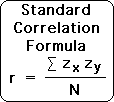
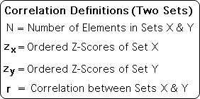
 Following is a standard formula for the correlation coefficient of 2 ordered data sets. For the correlation to have any utility in terms of prediction, both data sets must have a ‘normal’ bell curve distribution. The correlation is represented by ‘r’, while ‘N’ is the number of elements in each data set. Because data sets X and Y are ordered, their elements are paired. As such, N is also the number of ordered pairs.

‘Zx’ and ‘Zy’ are the Z-scores of the respective data sets. Each element has a distinct Z-score relative to the entire data set. When all the Z-scores of the ordered pairs are multiplied, summed up, and then divided by N, this yields the correlation ‘r’.

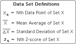
What is the Z-score? Let’s start with the following definitions for data set X. These are traditional notations, with the exception of the standard deviation. Although we have chosen a different notation for the standard deviation for reasons that will eventually become apparent, it is computed in the same fashion.

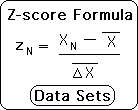
To determine the Z-score for any element of data set X, simply subtract the data set’s average from the data point and then divide by the standard deviation of the data set. This mathematical relationship is shown in the following formula. The Z-score determines how far beyond the average value that the element is. If a set has a normal distribution, some 70% of elements are within 2 standard deviations of the mean average and over 90% of the elements are within 3 standard deviations.

Now that we know what the Z-score is, we can better understand the mathematical correlation of a data set. Following are some standard definitions.

Following is the standard correlation formula that we discussed above.

The Living Correlation of a Data Stream

There is one primary difference between a data stream and a data set. A data stream is ongoing, while a data set has a fixed size with fixed elements. Statisticians compute measures that determine the nature of an entire data set, while data stream measures determine the nature of individual moments in the stream. In other words, data streams don’t have averages or standard deviations. However, individual moments in a data stream have averages and deviations.

In similar fashion, statisticians calculate measures that determine the correlation between two data sets. In contrast, data stream correlations refer to individual moments rather than the entire data stream. Because of the focus upon the dynamic nature of moments, data stream measures are particularly useful to living systems. They act as predictive descriptors, in that the measures both describe the current moment and predict what is coming next.

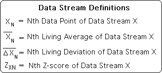
As such, data stream definitions deal with moments rather than the entire set. Following are some initial data stream definitions that parallel the data set definitions listed above. Note that both the Living Average and Living Deviation have a subscript to indicate which moment they refer to. 

Employing these definitions, we can determine the Living Z-score at each moment in the data stream according the following formula. The formula is identical to the data set formula with one major difference. The Average and Deviation refer to the former moment rather than the entire set.

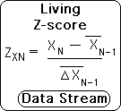
In similar fashion to the equivalent data set measures, the data stream’s Z-scores determine how much the current data point deviates from the average. Subtract the past average from the current data point and divide by the past deviation. The past average indicates the probable location of the next data point, while the past deviation determines the probable range. Just as with the data stream measure, a Living Z-score of 1 and below is considered normal, between 1 and 2 is considered unusual, while above 2 would be abnormal, definitely outside the probable range.

However, there is a major difference between the Z-score of a data set and the Living Z-score of a data stream. A data set must have a normal distribution for the Z-score to have well-defined limits. Living systems don’t have the luxury of time to make decisions that are relevant to immediate survival, for instance capturing prey and avoiding becoming prey. As such the Living Z-score applies to any data stream, no matter how erratic. Again precision is sacrificed for immediate relevance.

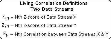
Now that we have a formula for the Z-score of a data stream, we can determine a formula for the Living Correlation between 2 data streams. Let’s start with some definitions. Again note that the correlation, R, has a subscript to indicate that it applies to an individual moment, not to the entire relationship between 2 data stream. Again this sense of individual immediacy is crucial information for living systems.

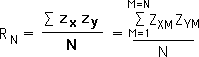
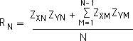
We begin with the standard formula for a correlation. In this case only, the subscript N on R indicates that it applies to 2 data sets with N elements. In other words, there are N ordered pairs. We then elaborate the formula with values for the summation. Just as before we take the product of the Z-scores of the ordered pairs from 1 to N, sum them up, and then divide by N to obtain the correlation.

Equation 1:

We then break the fraction into 2 parts by taking out the Nth product from the summation. The summation now only goes to N-1 rather than N.

Equation 2:

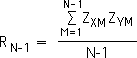
If we take out the Nth ordered pair from our data sets, the correlation of the truncated data sets would be determined by the following formula. Note that the denominator and summation limits are both reduced by 1 from Equation 1.

Equation 3:

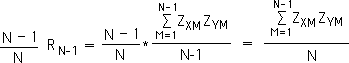
Multiply both halves of Equation 3 by N-1/N. Then cancel out the N-1 term.

Equation 4:

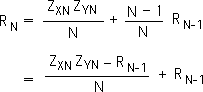
The term on the right of Equation 4 is identical to term on the right of Equation 2. We substitute the left term of Equation 4 into Equation 2. We then perform a standard algebraic procedure to obtain the bottom equality. Note: we have not changed the formula for the correlation coefficient of two data sets. We have just written it in a form that is more applicable to data streams. 

We now must convert this data stream formula into a data stream formula. As mentioned, data streams are ongoing. They do not have a distinct size. The subscripts refer to the moment N in the data stream, not the number of elements. It would be inappropriate to divide by a position. As with other data stream measures, we divide by D the Decay Factor, instead of N the number of elements in the stream. We have discussed both the practicality and utility of this constant in other papers.

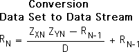
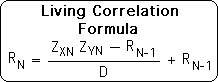
This is our formula for the Living Correlation. Reiterating, this data stream measure applies to moments, not the entire stream. To determine the present correlation: subtract the past correlation from the product of the current Z-scores, divide by D, the Decay Factor, and then add the past correlation.

Check out the next article for the practical applications of the Living Correlation.